The Dunford-Taylor representation of regularly accretive operators (here Laplacian) $$ (-\Delta)^{-s} = \frac{1}{2\pi i}\int_{C} z^{-s} (z+\Delta)^{-1}dz, \qquad 0 < s < 1, $$ where \(C\) is an appropriate contour in the complex plane, leads to numerical method for the approximation of the spectral and integral fractional laplacian.
Let \(\Omega\) be a bounded Lipschitz domain. The spectral fractional Laplacian \((-\Delta)^s\) with \(s\in (0,1)\) is defined for \(v\in \{w\in L^2(\Omega) : (-\Delta)^s w\in L^2(\Omega) \}\) by $$(-\Delta)^s v = \sum_{j=0}^\infty \lambda_j^s (v,\psi_j) \psi_j,$$ where \((\cdot,\cdot)\) denotes the \(L^2\) inner product and \(\{\psi_j\}\) is an orthonormal basis of eigenfunctions of \(-\Delta\) correspondin g to eigenvalues \(\{\lambda_j\}\).
We denote by \(H^s(\Omega) := (L^2(\Omega), H^1_0(\Omega))_{s,2}\) the interpolation space (real method). Given \( f \in L_2(\Omega)\), we seek to approximate \(u \in H^s(\Omega)\) satisfying $$(-\Delta)^{s} u = f \quad \textrm{in } \Omega.$$ The proposed approximation method relies on the so-called Balakrishnan formula $$ u = (-\Delta)^{-s} f = \frac{c_s}{2} \int_{0}^{\infty} \mu^{-s} (\mu I-\Delta)^{-1}f \,d \mu = c_s \int_{-\infty}^{\infty} e^{2st} (I-e^{2t}\Delta)^{-1}f \,d t,$$ where \(c_s:={2\sin(\pi s)}/{\pi}\), and consists in two steps:
The resulting \(N_- + N_+ + 1\) finite element problems are mutually independent, making the parallel implementation straightforward. In addition, for each subproblem it only requires the implementation of a classical finite element solver for the diffusion-reaction problem.
The discrepancy between the exact solution and its approximation consists of the sinc quadrature error, which is exponentially convergent, and the finite element approximation error, which is optimal up to a logarithmic factor depending on the smoothness of the data \(f\). It is worth mentioning that the error analysis does not require the domain to be convex.
For \(u,\varphi\in H^s(\Omega)\), the inner product also has an integral representation $$a_s(u,\varphi):=\int_\Omega (-\Delta)^{s/2} u (-\Delta)^{s/2}\varphi = \frac{c_s}{2} \int_{-\infty}^{\infty} e^{st} \int_\Omega \Big((-\Delta)(e^tI - {\Delta})^{-1} u\Big)\varphi dt.$$ The numerical approximation to the inner product follows essentially the same two steps as in the spectral fractional operator approximation.
The error estimation is achieved by analyzing the consistency error between \(a_s(u,\varphi)\) and its two-step numerical approximation. The consistency error is the sum of the exponentially convergent sinc quadrature error and the finite element error. A Strang's lemma type argument is used to derive error estimates.
The integral fractional Laplacian is defined using the Fourier transform. For \(v\) in the Schwartz space, the integral fractional Laplacian is a pseudo-differential operator with symbol \(|\zeta|^{2s}\), $$\mathscr{F} ((-\Delta)^s v)(\zeta) = |\zeta|^{2s}\mathscr{F}(v)(\zeta),$$ with \(\mathscr{F}\) denoting the Fourier transform. The definition can be extended to the Sobolev space \( H^s(\mathbb R^d)\) by a density argument.
Consider the following model problem involving the integral fractional Laplacian: given \(f\in L^2(\Omega)\), find \(u\in H^s(\Omega)\) satisfying $$ (-\Delta)^s \tilde{u} = f \qquad\;\text{in}\; \Omega, $$ where \(\tilde u\) denotes the extension by zero outside the domain \(\Omega\). Unlike the spectral fractional Laplacian, we could not find a useful integral representation of \(\tilde u\). Instead, the approximation relies on a formulation of the scalar product similar to the spectral case $$ \int_{\mathbb R^d} (-\Delta)^{s/2} \tilde u (-\Delta)^{s/2}\tilde\varphi = \frac{c_s}{2} \int_{-\infty}^{\infty} e^{st} \int_\Omega \Big( (-\Delta)(e^tI-\Delta)^{-1}\tilde u \Big) \varphi~ dt, $$ with \(u,\varphi\) in \(H^s(\Omega)\). This integral representation suggests the following approximation strategy similar to the one for the spectral Laplacian above:
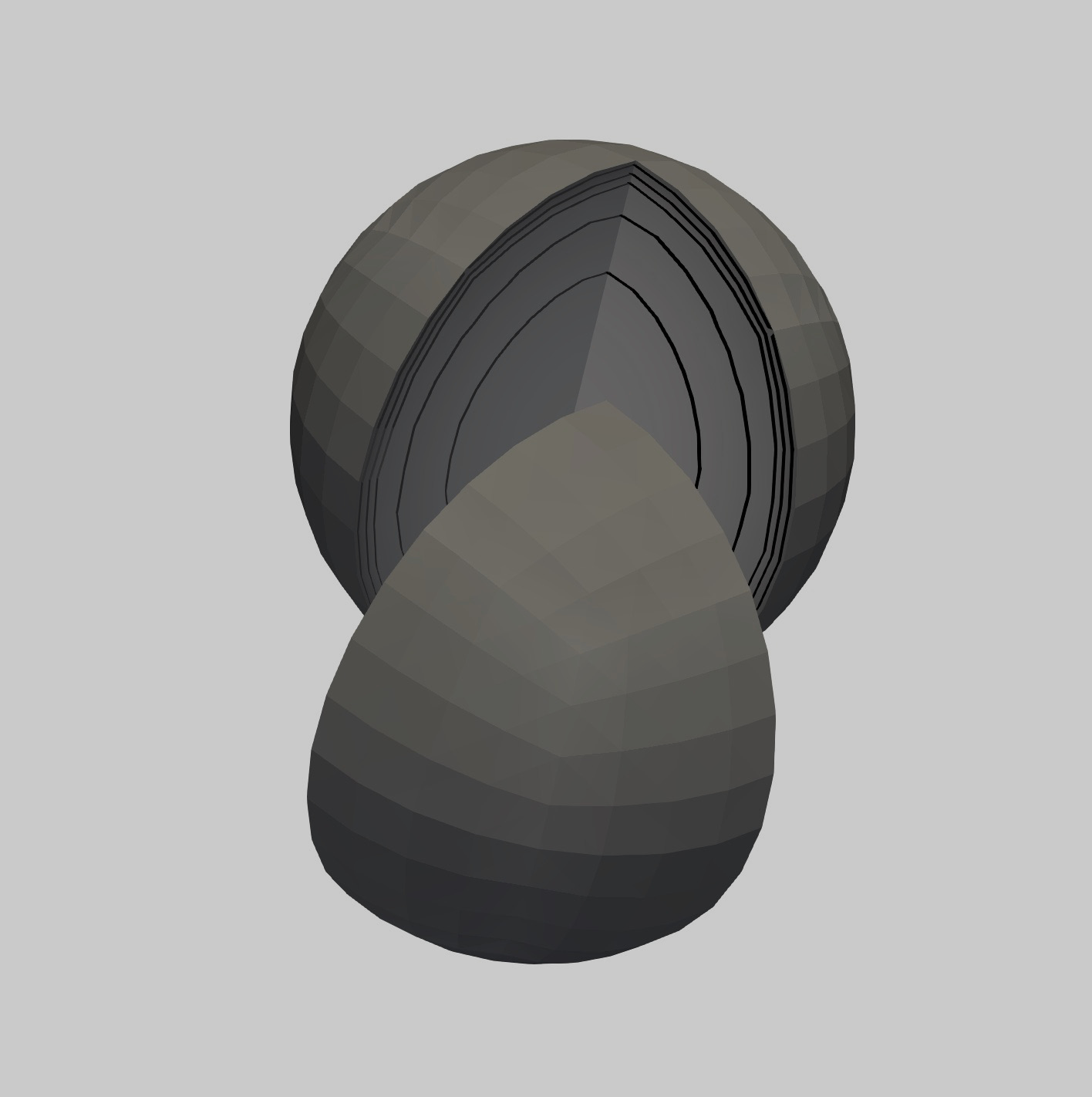
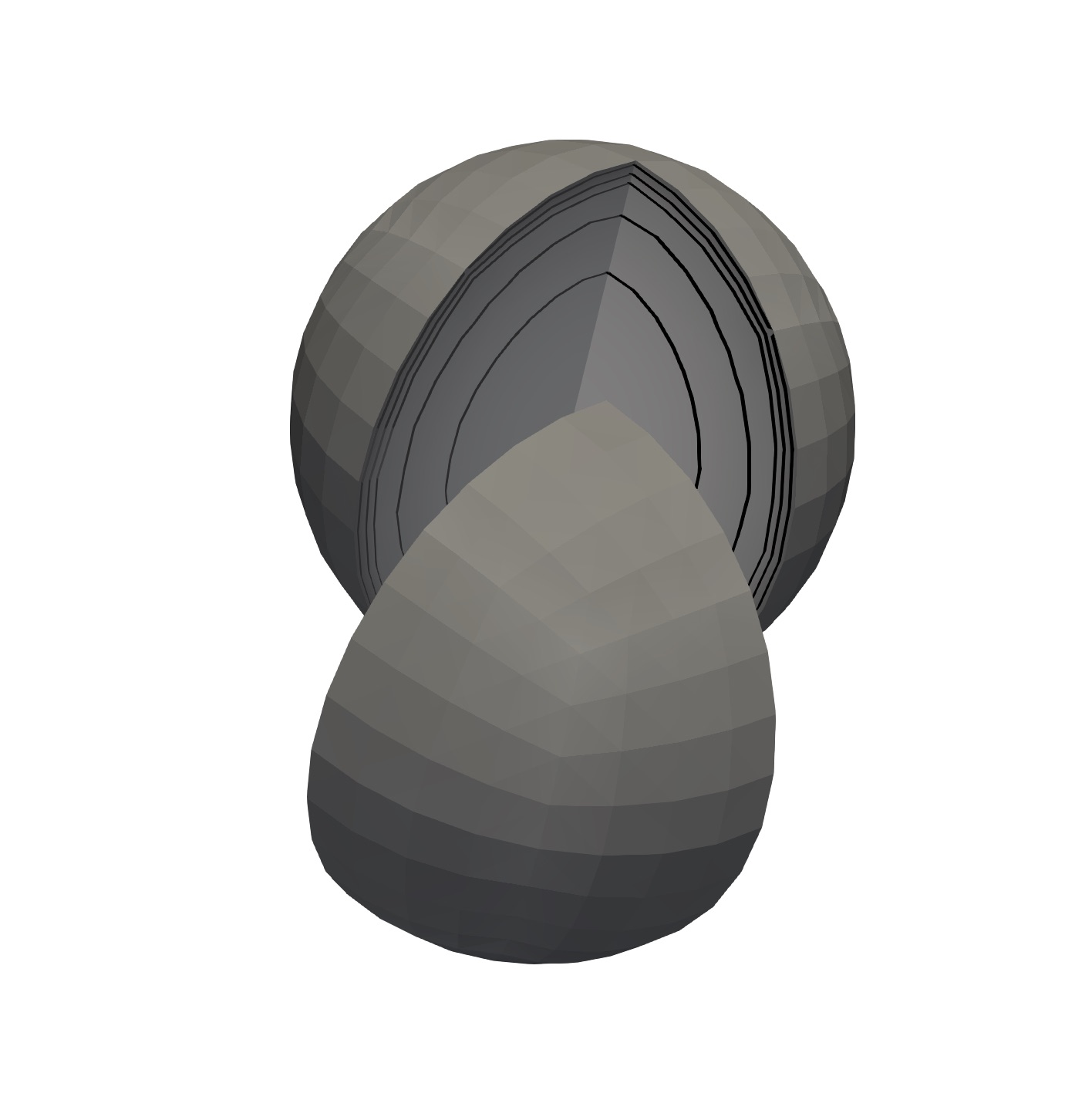
The discrepancy between the exact solution and its fully discrete approximation consists of three parts: an exponentially convergent sinc quadrature error, an exponentially convergent domain truncation error, and a finite element approximation error. The algorithm does not require \(\Omega\) to be convex and works on three dimensional domain as illustrated in the figure below.
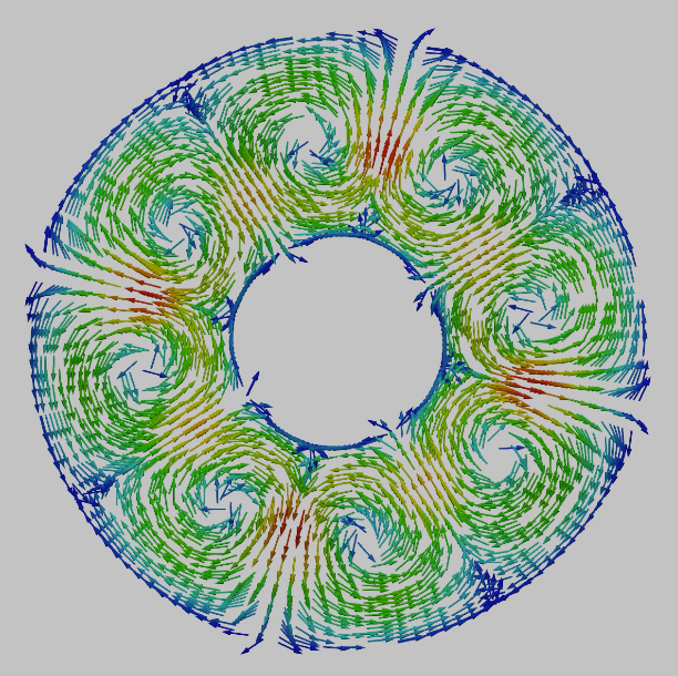
The electrical convection, or electroconvection in short, is the phenomenon caused by the application of a sufficiently large voltage difference across a thin-layer fluid such that the unbalanced charges are pushed by the applied electric field to form pairs of vortices of flows.
In the physical experiments by Tsai et al. (2007), at the room temperature the liquid crystal is at smectic-A stage so that the cigar-shaped molecules are arranged into layers. Within each layer, the molecules are aligned perpendicular to the plane of the film. Under such arrangement, the molecules are free to move along the film while movements normal to the layers are prevented. This leads to a two dimensional motion.
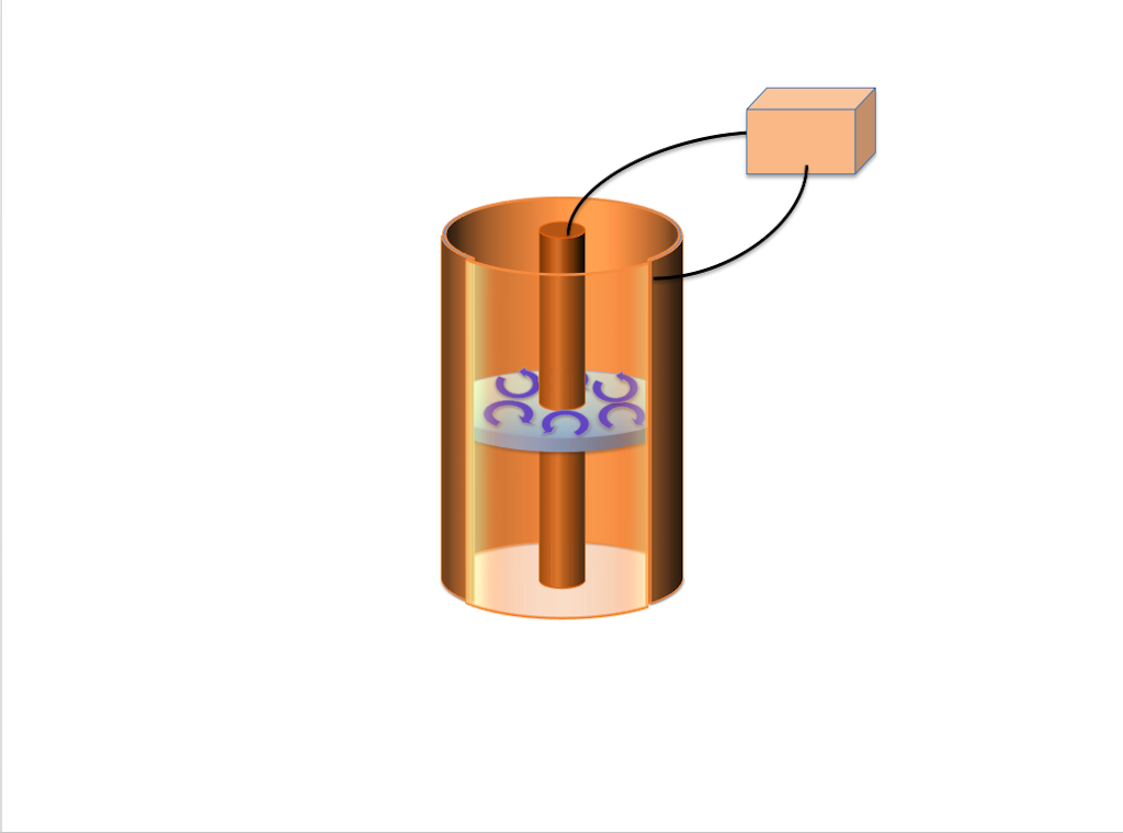
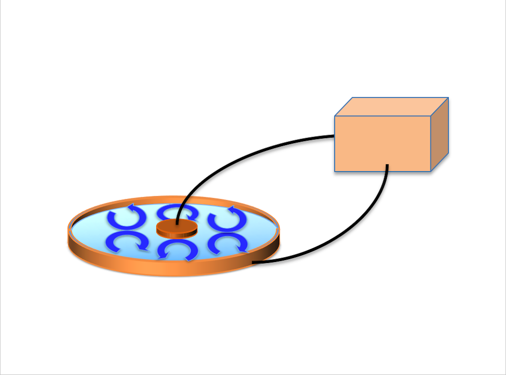
This thin-layered film is placed in between two concentric electrodes with the boundaries touching the electrodes. The inner electrode is charged with positive voltage \(V\) and the outer one is grounded. Inside the film, the positive charges are gathering near the inner boundary, while negative charges gather around the outer boundary. Such unstable equilibrium can be easily broke by a small perturbation on the charge distribution. As a consequence, counter-rotating vortex flows emerge when \(V\) exceeds an threshold value \(V_c\).
As in Tsai et al. (2007), we consider two settings: the electrodes extend to infinity in the normal direction or the electrodes have negligible thickness, see Figure 1. The former corresponds to the simulation reported in (Tsai 2007, Tsai et al. 2007) while the later is related to the analysis by Constantin et. al. (2016). A model reduction to the fluid domain introduces nonlocal representation for the electric potential \(\Psi:\Omega \to \mathbb R\) either involving the spectral fractional Laplacian (infinite electrodes): $$ (-\Delta)^{1/2} \Psi = q \quad \textrm{in } \Omega, $$ or the integral fractional Laplacian (slim electrodes): $$ (-\Delta)^{1/2} \tilde\Psi = q + g \quad \textrm{in } \Omega. $$ Here \(q:\Omega \to \mathbb R\) is the liquid surface charge density, and \(g:\Omega \to \mathbb R\) is an axis-symmetric function accounting for the voltage difference.
The electric potential \(V\) and the aspect ratio between the inner radius and outer radius of the film are critical parameters for electroconvection to develop.
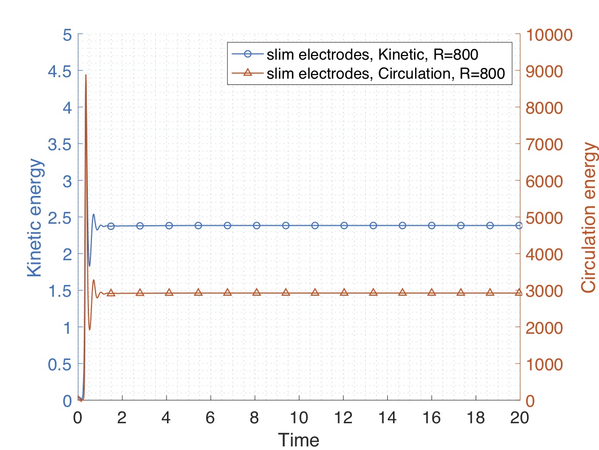
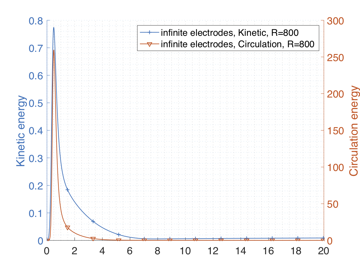
The difference between the two models is strikingly significant. To illustrate this claim, we consider an aspect ratio of \(0.33\), a Rayleigh number of \(\mathcal R=800\), a Prandtl number of \(\mathcal P = 10\) and provide in Figure 2 a comparison of the evolution of kinetic and circulation energies $$ E_k := \frac{1}{2}\int_{\Omega} |\mathbf u|^2 \;d\mathbf x, \qquad E_{curl} := \int_{\Omega} |\nabla\times \mathbf u|^2 \;d\mathbf x, $$ where \(\mathbf u\) denotes the velocity field of the fluid.
We investigate the effect of the geometry.
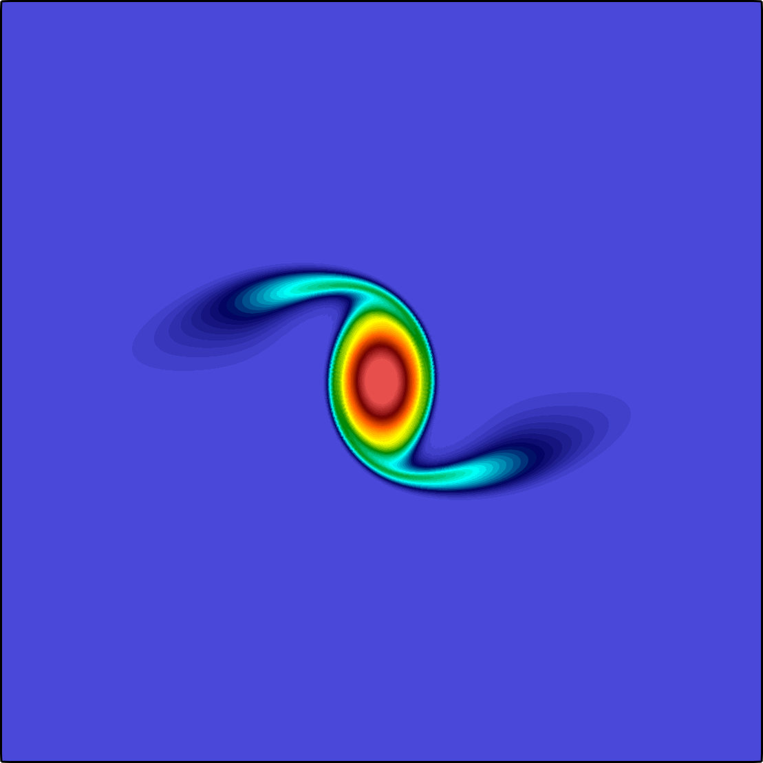
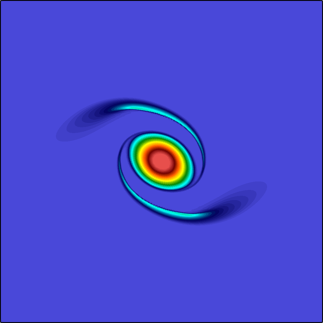
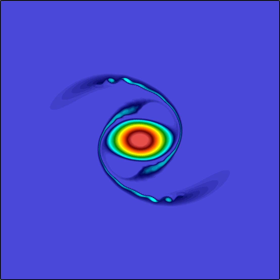
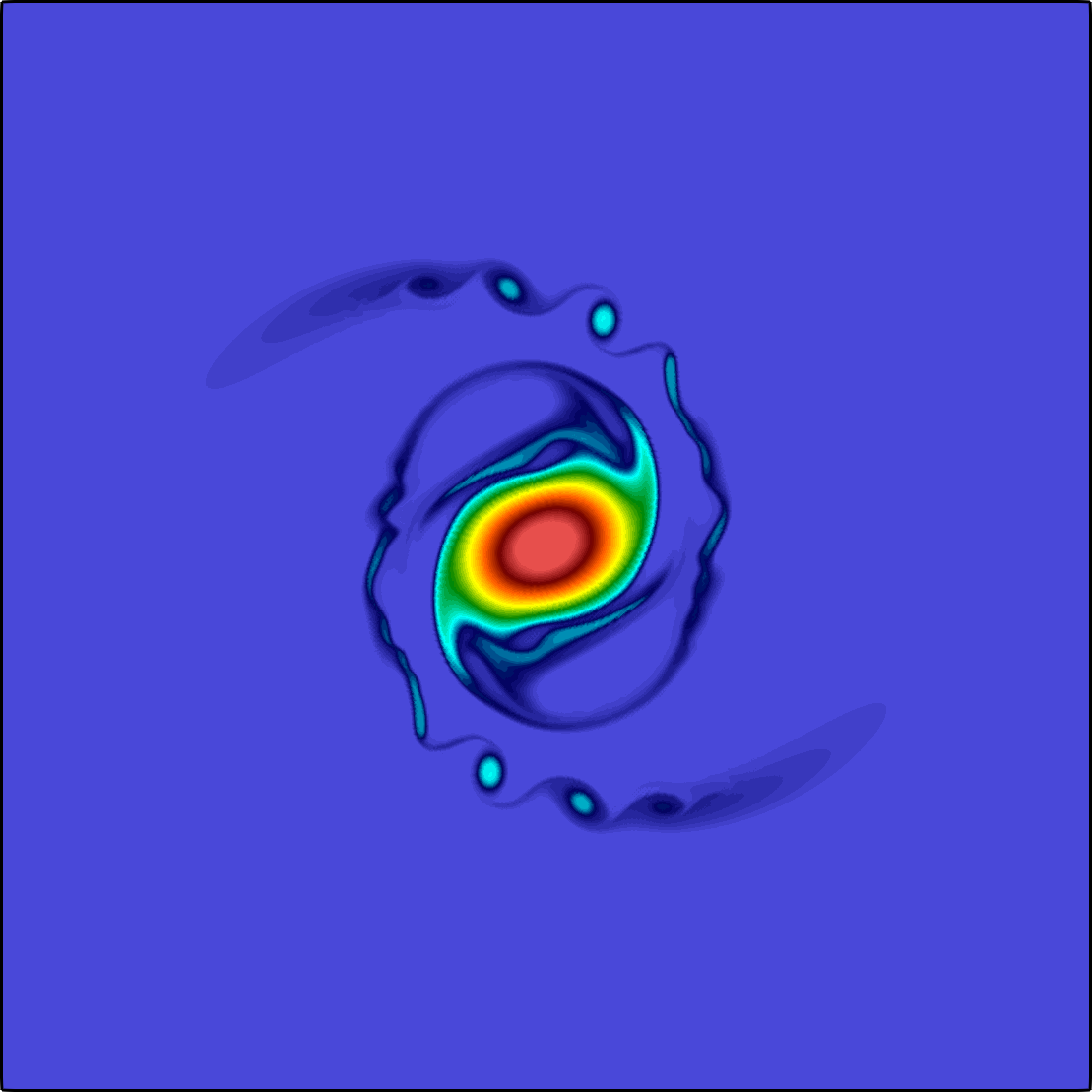
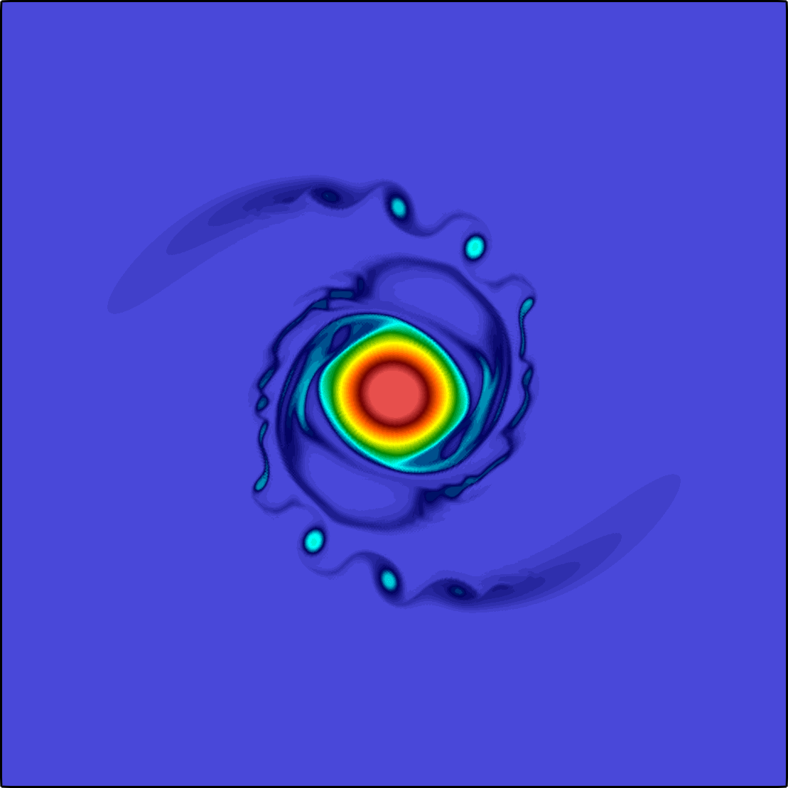
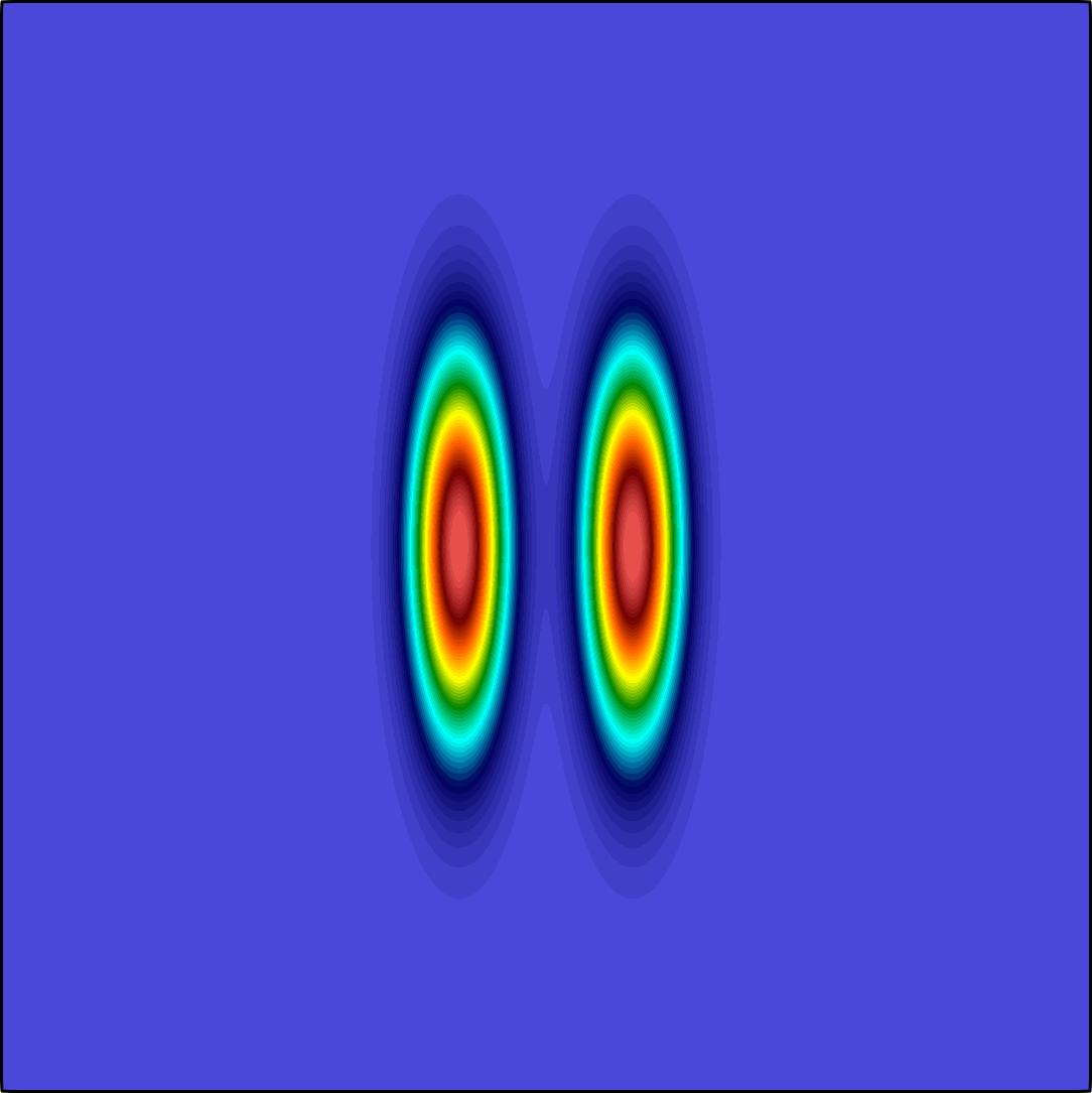
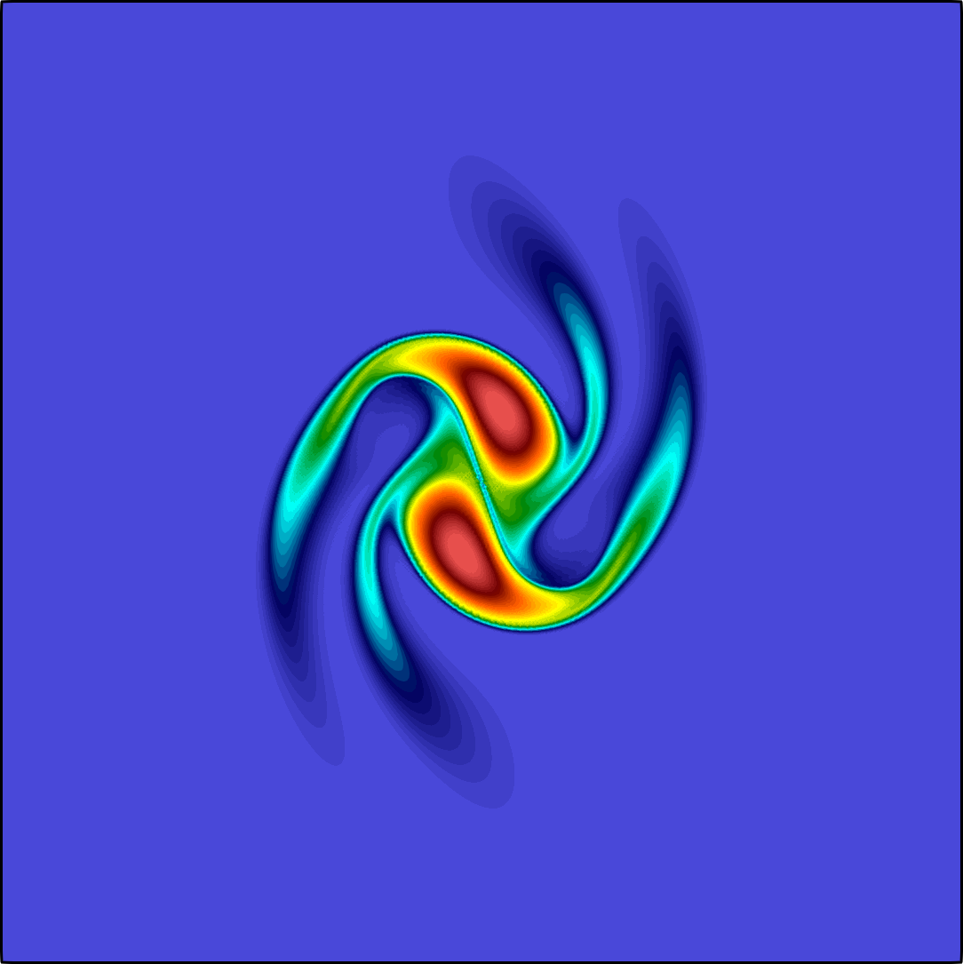
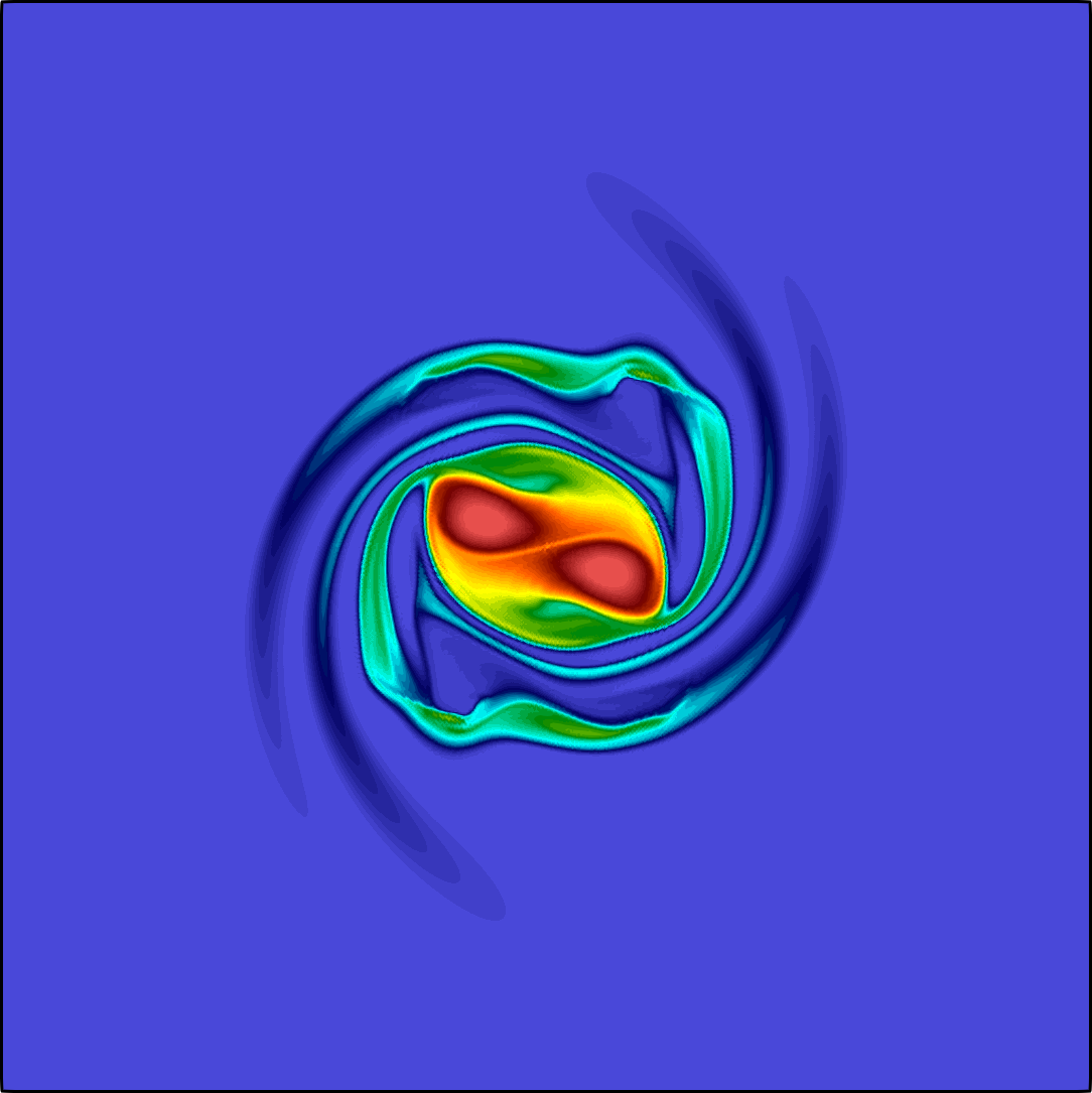
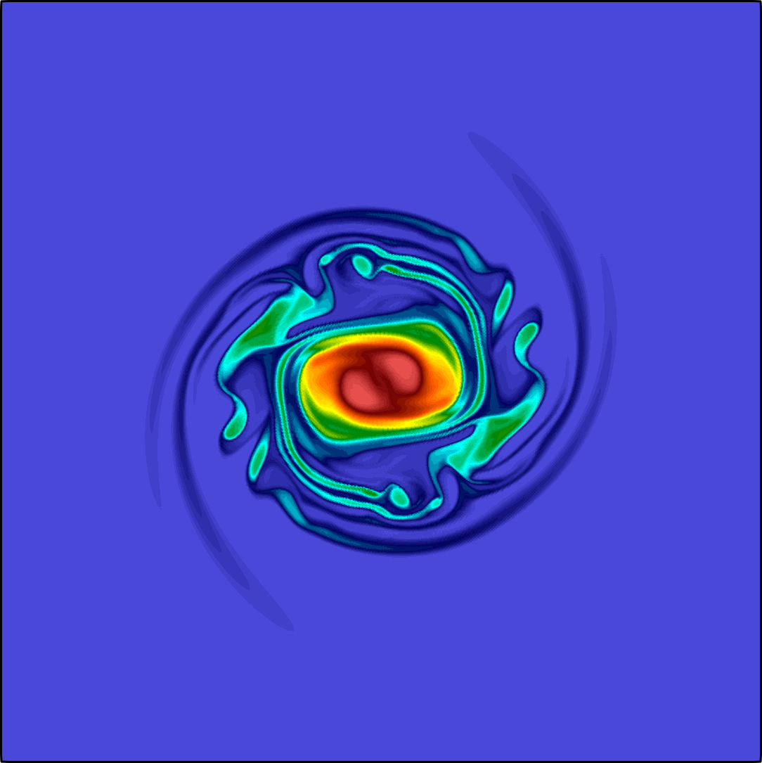
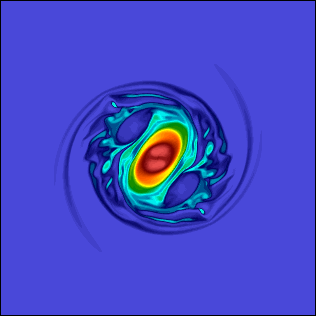
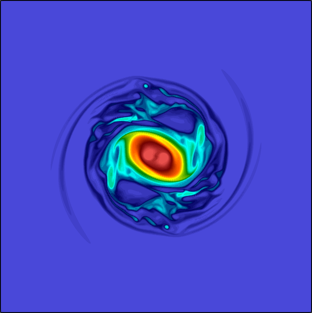
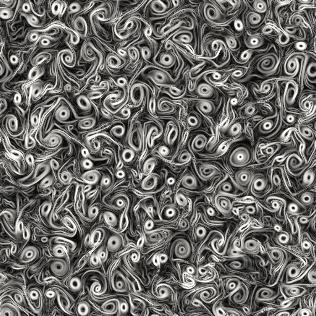
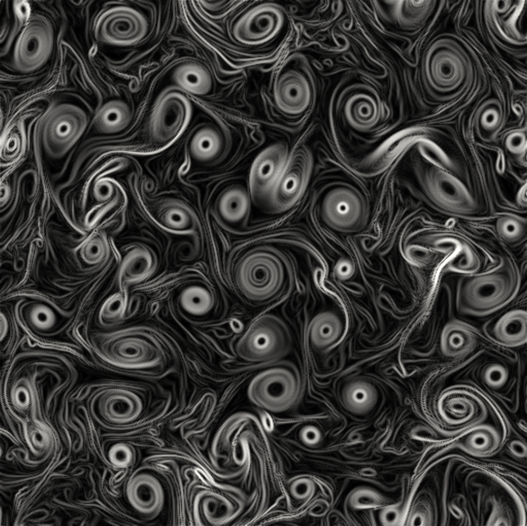
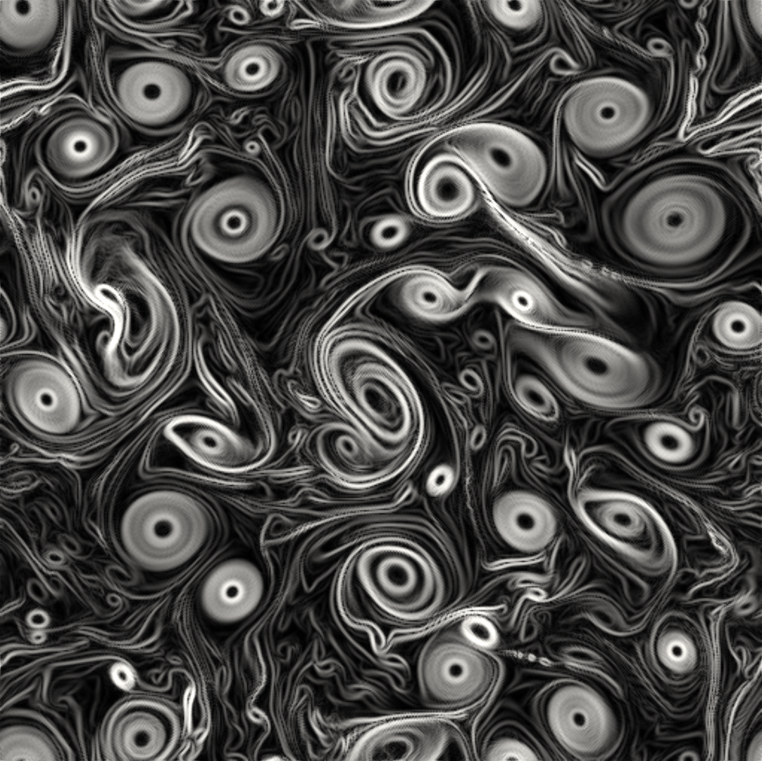
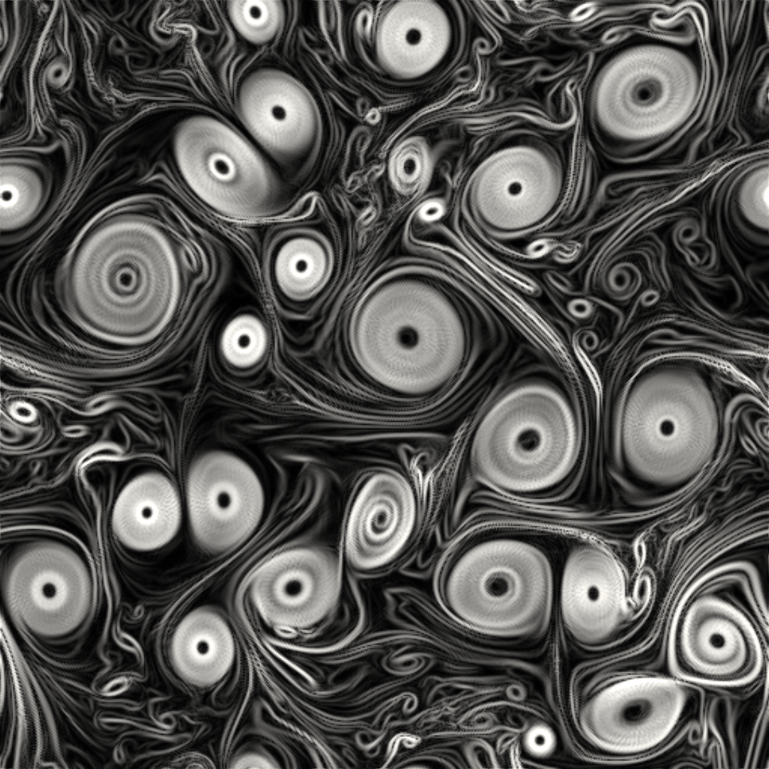
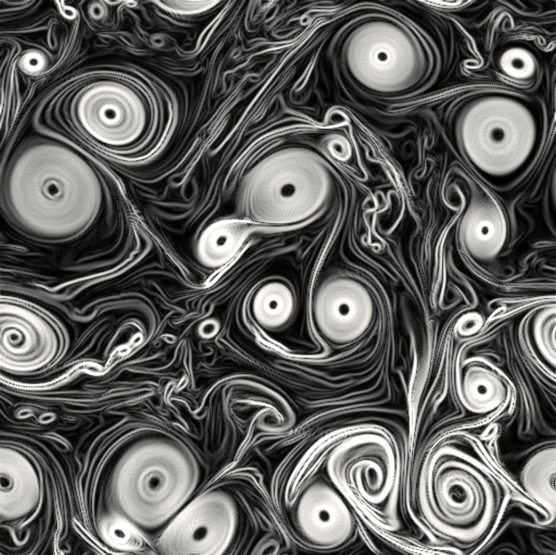
The general quasi-geostrophic model, first introduced by J. G. Charney in the 1940s, has been very successful for the study of oceanic and atmospheric dynamics in the mid-to-high latitude region of the earth where the Coriolis effect is significant. The characteristic property of the quasi-geostrophic system is the conservation of potential vorticity along the geostrophic flow. If in addition to the potential vorticity conservation, the assumption on the potential temperature conservation reduces the model to the surface quasi-geostrophic equation (Constantin et al. 1994,Held et al. 1995)
The governing equation is a transport equation with a fractional dissipation term: $${\partial_t \theta} + \mathbf{u}\cdot \nabla \theta + \kappa(-\Delta)^{s}\theta = 0, \quad \textbf{u} = \nabla^{\bot}\psi, \quad (-\Delta)^{1/2} \psi= -\theta \quad\text{ all in }\; \Omega.$$ Here \(\Omega\) is a square domain sitting on the \(xy\) plane, the potential temperature \(\theta = \theta(\mathbf{x},t)\) is a scalar function defined on \(\Omega\times[0,\texttt T]\) with \(\texttt T>0\), \(\nabla^{\bot}\psi := (-\partial_y \psi, \partial_x \psi)^T\), and \(\psi:\Omega\times[0,\texttt T]\to \mathbb R\) is the geopotential. The fractional power \(s\) belongs to \([1/2,1)\), and the coefficient \(\kappa \ge 0\) is a constant. Both \(\psi\) and \(\theta\) are supplemented with periodic boundary condition, and further fixed by an averaging constraint. Both fractional operators are spectral fractional Laplacians. The non-local property of the fractional term is the main difficulty in both analysis and numerical approximation.
The expression of the velocity \(\textbf{u}\) corresponds to the motion along the iso-bars of \(\psi\). This is due to the fact that the gradient pressure is balanced by the Coriolis force in the gradient direction. For instance, for a high-pressure area in the southern hemisphere, the pressure gradient is pointing outward, while the Coriolis force is perpendicular to the direction of the movement to the left side, leading to a counter-clockwise rotation to balance the two forces. The term \(\kappa(-\Delta)^{s}\theta\) is the so-called Ekman pumping, representing a balance between the vertical component of the Coriolis force and vertical frictional force. Typically, \(\kappa > 0\) and \(s = 1/2\).